Measuring What Matters: Objective Metrics for Image Generation Assessment


Generating high-quality visuals with state-of-the-art models is now more and more accessible. Open-source models run on laptops, and cloud services turn text into images in seconds. These models are already reshaping industries like advertising, gaming, fashion, and science.
But creating images is the easy part. Judging their quality is much harder. Human feedback is slow, expensive, biased, and often inconsistent. Plus, quality has many faces: creativity, realism, and style don’t always align. Improving one can hurt another.
That’s why we need clear, objective metrics that capture quality, coherence, and originality. we’ll look at ways to measure image quality and compare models with Pruna, beyond just "does it look cool?"
Metrics Overview
There is no single correct way to categorize evaluation metrics, as a metric can belong to multiple categories depending on its usage and the data it evaluates. In our repository all quality metrics can be computed in two modes: single and pairwise.
- Single mode evaluates a model by comparing the generated images to input references or ground truth images, producing one score per model.
- Pairwise mode compares two models by directly evaluating the generated images from each model together, producing a single comparative score for these two models.
This flexibility enables both absolute evaluations (assessing each model individually) and relative evaluations (direct comparisons between models).
On top of the evaluation modes, it also makes sense to think about metrics in terms of their evaluation criteria to provide structure and clarity. Our metrics fall into two overarching categories:
- Efficiency Metrics: Measure the speed, memory usage, carbon emissions, energy, etc. usage of models during inference. At pruna, we focus on making your models smaller, faster, cheaper, greener, so evaluating your models using these efficiency metrics is a natural fit. However, because efficiency metrics are not specific to image generation tasks, we won't discuss them in detail in this blog post. If you'd like to learn more about these metrics, please refer to our documentation.
- Quality Metrics: Measure the intrinsic quality of generated images and their alignment to intended prompts or references. These include:
- Distribution Alignment : How closely generated images resemble real-world distributions.
- Prompt Alignment : Semantic similarity between generated images and their intended prompts.
- Perceptual Alignment : Pixel-level or perceptual similarity between generated and reference images.
The table below summarizes the most common quality metrics available at pruna, their categories, score ranges, and key limitations to help guide metric selection.
| Metric | Measures | Category | Range (↑ higher is better/↓ lower is better) | Limitations |
|---|---|---|---|---|
| FID | Distributional similarity to real images | Distribution Alignment | 0 to ∞ (↓) | Assumes Gaussianity, requires large dataset, depends on a surrogate model |
| CMMD | CLIP-space distributional similarity | Distribution Alignment | 0 to ∞ (↓) | Kernel choice affects results, depends on a surrogate model |
| CLIPScore | Image-text alignment | Prompt Alignment | 0 to 100 (↑) | Insensitive to image quality, depends on a surrogate model |
| PSNR | Pixel-wise similarity | Perceptual Alignment | 0 to ∞ (↑) | Not well perceptually aligned |
| SSIM | Structural similarity | Perceptual Alignment | -1 to 1 (↑) | Can be unstable for small input variations |
| LPIPS | Perceptual similarity | Perceptual Alignment | 0 to 1 (↓) | depends on a surrogate model |
Distribution Alignment Metrics
Distribution alignment metrics measure how closely generated images resemble real-world data distributions, comparing low and high features. In pairwise mode, they compare outputs from different models to produce a single score that reflects relative image quality.

The generated image closely resembles the real one, and the distributions are well aligned, suggesting good quality.

the generated image is noticeably off, and the distributions differ significantly, which the metric captures as a mismatch.
Fréchet Inception Distance (FID): FID (introduced here) is one of the most popular metrics for evaluating how realistic AI-generated images are. It works by comparing the feature distribution of the reference images (e.g. real images) to the images generated by the model to evaluate.
Here’s how it works in a nutshell:
- We take a pretrained surrogate model and pass both real and generated images through it. The pretrained surrogate model is usually the Inception v3 explaining the metric name**.**
- The model turns each image into a feature embedding (a numerical summary of the image). We assume the embeddings from each set form a Gaussian distribution.
- FID then measures the distance between the two distributions — the closer they are, the better.
A lower FID score indicates that the generated images are more similar to real ones, meaning better image quality.
Want the math?
FID is calculated as the Fréchet distance between two multivariate Gaussians:
FID = ||μr − μg||² + Tr(Σr + Σg − 2(Σr Σg)1/2)Where:
- (μr, Σr) are the mean and covariance of real image features.
- (μg, Σg) are the mean and covariance of generated image features.
- Tr denotes the trace of a matrix.
- (Σr Σg)1/2 represents the geometric mean of the two covariance matrices.
Clip Maximum-Mean-Discrepancy (CMMD): CMMD (introduced here) is another way to measure how close your generated images are to real ones. Like FID, it compares feature distributions, but instead of using Inception features, it uses embeddings from a pretrained CLIP model.
Here’s how it works:
- We take a pretrained surrogate model and pass both real and generated images through it. The pretrained surrogate model is usually the CLIP.
- The model turns each image into a feature embedding (a numerical summary of the image). We do not assume the embeddings from each set form a Gaussian distribution.
- Use a kernel function (usually RBF) to compare how these distributions differ, without assuming they are Gaussian.
A lower CMMD score indicates that the feature distributions of generated images are more similar to those of real images, meaning better image quality.
Want the math?
CMMD is based on the Maximum Mean Discrepancy (MMD) and is computed as:
CMMD = 𝔼[ k(φ(xr), φ(x′r)) ] + 𝔼[ k(φ(xg), φ(x′g)) ] − 2𝔼[ k(φ(xr), φ(xg)) ]Where:
- φ(xr) and φ(x′r) are two independent real image embeddings extracted from CLIP.
- φ(xg) and φ(x′g) are two independent generated image embeddings extracted from CLIP.
- k(x, y) is a positive definite kernel function that measures similarity between embeddings.
- The expectations 𝔼[·] are computed over multiple sample pairs.
Prompt Alignment Metrics
Prompt alignment metrics evaluate how well generated images match their input prompts, especially in text-to-image tasks. In pairwise mode, they instead measure semantic similarity between outputs from different models, shifting focus from prompt alignment to model agreement.
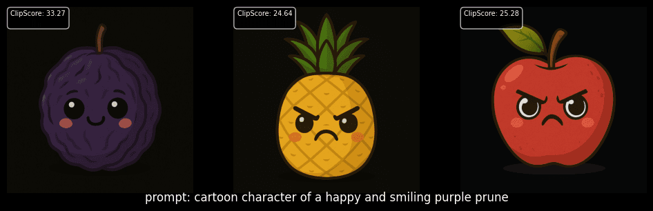
CLIPScore: CLIPScore (introduced here) tells you how well a generated image matches the text prompt that produced it. It uses a pretrained CLIP model, which maps both text and images into the same embedding space.
Here’s the idea:
- Pass the image and its prompt through the surrograte CLIP model to get their embeddings.
- Measure how close these two embeddings. The closer they are, the better the alignment between the image and the prompt.
CLIPScore ranges from 0 to 100. A higher score means the image is more semantically aligned with the prompt. Note that this metric doesn’t look at visual quality, just the match in meaning.
Want the math?
Given an image x and its corresponding text prompt t, CLIP Score is computed as:
CLIPScore = max⎛100 × (φI(x) · φT(t)) / (||φI(x)|| · ||φT(t)||), 0⎞Where:
- φI(x) is the CLIP image embedding of the generated image.
- φT(t) is the CLIP text embedding of the associated prompt.
CLIP Score ranges from 0 to 100, with higher scores indicating better alignment between the image and its prompt. However, it may be insensitive to image quality since it focuses on semantic similarity rather than visual fidelity.
Perceptual Alignment Metrics
Perceptual alignment metrics evaluate the perceptual quality and internal consistency of generated images. They compare pixel-level or feature-level differences between images. These metrics are often pairwise by nature, as comparing generated images with other generated images is more appropriate in certain cases, such as pixel-by-pixel comparisons.
Peak Signal-to-Noise Ratio (PSNR): PSNR measures the pixel-level similarity between a generated image and its reference (ground truth) image. It is widely used for evaluating image compression and restoration models.
A higher PSNR value indicates better image quality, but PSNR does not always correlate well with human perception.
Want the math?
PSNR is computed as:
PSNR = 10 × log10 ⎛ (L²) / MSE ⎞Where:
- L is the maximum possible pixel value (e.g., 255 for an 8-bit image).
- MSE (Mean Squared Error) is the average squared difference between pixel values.
Structural Similarity Index (SSIM): SSIM improves upon PSNR by comparing local patterns of pixel intensities instead of just raw pixel differences. It models human visual perception by considering luminance, contrast, and structure in small image patches
SSIM ranges from -1 to 1, where 1 indicates perfect similarity.
Want the math?
SSIM is often computed as:
SSIM(x, y) =
(2μxμy + C1)(2σxy + C2) / (μx2 + μy2 + C1)(σx2 + σy2 + C2)Where:
- μx, μy are the mean intensities of images x and y.
- σx2, σy2 are the variances.
- σxy is the covariance between the images.
- C1, C2 are small constants for stability.
Learned Perceptual Image Patch Similarity (LPIPS): LPIPS is a deep-learning-based metric that measures perceptual similarity between images using features from a pre-trained neural network (e.g., VGG, AlexNet). Unlike PSNR and SSIM, LPIPS captures high-level perceptual differences rather than pixel-wise differences.
Want the math?
LPIPS is computed as:
LPIPS(x, y) = ∑l wl || Fl(x) − Fl(y) ||22Where:
- Fl(x) and Fl(y) are deep feature representations of images x and y from layer l.
- wl are learned weights that adjust the importance of each feature layer.
A lower LPIPS score means the generated image is more perceptually similar to the reference.
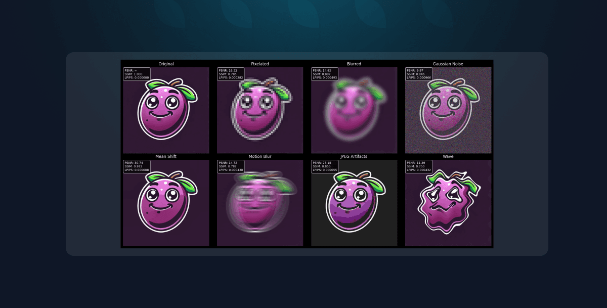
To illustrate how different distortions impact metric scores, let's look at the following example. The image below showcases various distortions applied to an original image and how metrics like SSIM, PSNR, and LPIPS react to these changes.

The results in the image illustrate how different types of distortions affect the scores given by these task-based metrics. Notably:
- Blurred images tend to score higher in SSIM than in PSNR. This suggests that while fine details are lost, the overall structure and patterns of the image remain intact, which aligns with SSIM’s focus on structural consistency.
- Pixelated images, on the other hand, maintain relatively high PSNR values but drop in SSIM ranking. This indicates that while pixel intensity differences remain small, the structural coherence of the image is significantly degraded—highlighting SSIM’s sensitivity to spatial relationships rather than just pixel-level accuracy.
These observations demonstrate why selecting the right metric is crucial. Each of the metrics captures different aspects of image quality, making them useful in different scenarios depending on the type of distortion and the perceptual quality being assessed.
Confidently evaluate AI models with the Evaluation Agent!
The evaluation framework in pruna consists of several key components:
Step 1: Define what you want to measure
Use the
Taskobject to specify which quality metrics you'd like to compute. You can provide the metrics in three different ways depending on how much control you need.from pruna.evaluation.task import Task from pruna.data.pruna_datamodule import PrunaDataModule from pruna.evaluation.metrics.metric_torch import TorchMetricWrapper # Method 1: plain text from predefined options evaluate_image_generation_task = Task("image_generation_quality", datamodule=PrunaDataModule.from_string('LAION256')) # Method 2: list of metric names metrics = ['clip_score', 'psnr'] evaluate_image_generation_task = Task(request = metrics, datamodule=PrunaDataModule.from_string('LAION256')) # Method 3: list of metric instances clip_score_metric = TorchMetricWrapper("clip_score", model_name_or_path = "openai/clip-vit-base-patch32") psnr_metric = TorchMetricWrapper('psnr', base=2.0) metrics = [clip_score_metric, psnr_metric] evaluate_image_generation_task = Task(request= metrics, datamodule=PrunaDataModule.from_string('LAION256'))Step 2: Run the Evaluation Agent
Pass your model to the
EvaluationAgentand let it handle everything: running inference, computing metrics, and returning the final scores.from pruna.evaluation.evaluation_agent import EvaluationAgent eval_agent = EvaluationAgent(evaluate_image_generation_task) results = eval_agent.evaluate(your_model)
As AI-generated images become more prevalent, evaluating their quality effectively is more important than ever. Whether you're optimizing for realism, accuracy, or perceptual similarity, selecting the right evaluation metric is key. With Pruna now open-source, you have the freedom to explore, customize, and even contribute new evaluation metrics to the community .
Our documentation and tutorials (here) provides a step-by-step guide on how to add your own metrics, making it easier than ever to tailor evaluations to your needs. Try it out today, contribute, and help shape the future of AI image evaluation!